The case for lifelong learning
 Lifelong learning (also known as continual learning) is the problem of learning multiple consecutive tasks in a sequential manner where knowledge gained from previous tasks is retained and used for future learning [1]. Living in a temporal world, we as humans absorb information in a sequential manner. Children in kindergarten for example learn the alphabet in a sequential manner: first 'A', then 'B', etc. Modern machine learning algorithms work really well in a batch-setting, i.e. when they are able to process all the data multiple times (generally through sub-sampled mini-batches). Most of the drastic advances in machine learning over the past years have been due to performance gains in deep supervised batch learning [2, 3, 4]. However, in order to transition models to more realistic scenarios such as the ones we as humans face on a day-to-day basis, we need to focus our efforts on lifelong learning. See [12] for a more eloquent and convincing argument on the topic.
This paradigm of learning contrasts traditional online learning algorithms [5] which generally try to find the best representation for the currently observed data. Lifelong Learning algorithms on the other hand posit that you need to remember all previous learning and leverage it for future scenarios, even if it is not useful at the current time frame. Online methods such as Streaming Variational Bayes[6] update the posterior distribution \(P(z | \mathrm{X}_1, ..., \mathrm{X}_t)\) of a model such that it best reflects the currently observed data using an update function : \(P(z | \mathrm{X}_1, ..., \mathrm{X}_t) \approx \mathcal{A}_t(\mathrm{X}_t, \mathcal{A}_{t-1})\). The problem with this formulation is that the previous data \(\mathrm{X}_{t-1}\) is not a present in the update function (except through the previous posterior \(\mathcal{A}_{t-1}\)). As we shall discuss shortly, this causes issues when using gradient descent based models.
The typical problem that occurs when utilizing a gradient-descent based model in a sequential manner is that of Catastrophic Forgetting [7]. This phenomenon appears when the model parameters start to become biased to the most recent samples observed, while forgetting what was learnt from older samples. Recently there have been a whole slew of methods that attempt to solve the problem; in our work we categorize these into four main strategies (note that this isn't all-encompassing) : transfer learning, replay mechanisms, parameter regularization and distribution regularization.
Requirements of a lifelong learner:
To be useful in a practical setting a lifelong learner needs to fulfill certain requirements, namely:
- Scalability: the models utilize need to scale to large datasets
- Finite memory footprint: it is not possible to store all of the observed data in a lifelong setting, so there needs to be a solution to address this problem. Storing a model per observed task is also not feasible.
- Evaluation strategies: as discussed in [8] most modern lifelong/continual learning evaluate one of two major dataset transitions: a set of split data-distributions that operate over a similar distribution space (eg: the digit '1' in MNIST to the digit '2'). The alternative is drastically different distributions such as MNIST -> Permuted MNIST. To be successful, a lifelong learner should be able to handle both of these and also transfer useful features/ speedup learning between similar tasks.
- Leverage previously learnt representations to improve future learning time (if applicable)
We observe that all of the current strategies such as Variational Continual Learning (VCL) [9], Elastic Weight Consolidation (EWC) [10], Learning without Forgetting [11] fail with respect to one of the above points; for example VCL adds a head-network per task which fails point #2 boiling the solution down to Progressive networks [13]. In addition VCL keeps a buffer of sampler per observed dataset which violates #1.
Lifelong VAE:
Our solution to the problem was three-fold:
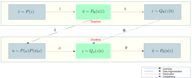
- Utilize a student-teacher architecture as a form of data replay
- Introduce a cross-model KL regularizer (called consistency regularizer) in the paper
- Introduce a decoupled discrete + continuous latent variable model along with a information gain regularizer
The teacher (top row) generates synthetic samples which are (conditionally) used by the student. Thus, the student observes either true data samples from the currently observed data or synthetic samples generated by the teacher. The sampling proportions are kept in check using the weights \(\pi\) of the student's input data distribution \(\mathrm{x} \sim P(\omega)P(\mathrm{x} | \omega), \, \omega \sim \text{Ber}(\pi) \). In the current work we assume we know when data distributions transition. In the future we hope to explore anomaly detection techniques to autonomously detect this, however avoid this here for the sake of preventing compounding errors . This is a pretty standard practice in all other works of lifelong / continual learning at this point in time. Making this assumption allows us to focus on the core problem of mitigating catastrophic interference, rather than an anomaly detection problem.
Bayesian Posterior Update:
In order allow the model to leverage previously learnt representations we take two steps:
- Introduce a Bayesian update rule \(KL(Q_{\Phi}(z\ |\ \mathrm{x}) || Q_{\phi}(z\ |\ \mathrm{x})) \) between the teacher, \(Q_{\Phi}\), and student posteriors, \(Q_{\phi}\).
- Enact an initial weight transfer from the teacher model to the student model when a distribution shift occurs.
In the paper we show that for isotropic gaussian and discrete distributions, that this posterior update rule is a natural extension of the ELBO over sequences of distributions, making the proposed regularizer in #1 derived from first principles and not an ad-hoc term. In our experiments we demonstrate that this regularizer aids in helping our model converge faster.
Latent Variable:
Our student model receives both real samples and synthetic samples generated by the teacher model. Recall that a standard VAE utilizes an isotropic gaussian posterior distribution and that VAEs generate data by sampling the prior ,\( P(z) \), and decoding the sample through \(P_{\theta}(x|z)\). The problem with a typical \(\mathcal{N}(0, 1)\) prior is that samples further away from the mean will get sampled less often. In a lifelong setting this scenario leads us again to catastrophic forgetting. To resolve this we model our posterior as an independent discrete + continuous latent variable:
\(Q_{\phi} ( z_d, z_c\ |\ x) = Q_{\phi} ( z_d\ |\ x) Q_{\phi} ( z_c\ |\ x) \)
The key idea here is that we want the discrete \(Q_{\phi} ( z_d\ |\ x) \) to represent the most discriminative aspects of the full posterior \(Q_{\phi} ( z_d, z_c\ |\ x) \). Nothing in the above formulation guarantees this.
Information Restricting Regularizer:
In order to enforce that \(z_d\) contain the most discriminative aspects of the posterior we introduce a negative information gain regularizer. This regularizer is similar to the one used in InfoGAN [18], but has a few key differences: namely we minimize the mutual information between \(\hat{x}\), the generated sample and \(z_c\), the continuous latent variable. Since our model doesn't have any skip connections, the only way for data to flow is through from \(x \mapsto [z_d, z_c] \mapsto \hat{x}\). Thus minimizing the mutual information between \( z_c \) and \(\hat{x}\) maximizes the mutual information between \(z_d\) and \(\hat{x}\). Finally, as opposed to InfoGAN, which uses the variational bound (twice) on the mutual information [14], our regularizer has a clear interpretation: it restricts information through a specific latent variable within the computational graph.
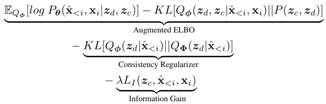
Optimization Objective:
Our final loss function ends up being:
Experiments:
Lifelong learning is a challenging area; coupling that with generative modeling makes the problem much more challenging. In such scenarios, simple datasets such as MNIST or FashionMNIST become extremely challenging. This is mainly due to the fact that we need to remember our previously learnt representation for data that we never observe in the future. As we add more and more distributions to our knowledge pool we will see a natural degradation of performance.
We validate our results on three datasets, namely: sequential single-object FashionMNIST, sequential permuted MNIST and finally experiment with a transfer learning scenario from MNIST \(\mapsto\) SVHN. We utilize two key metrics: the frechet distance as proposed by [15] and the negative test elbo (lower being better for both). We contrast our model to a baseline VAE, a full-batch VAE, a VAE that progressively adds datasets and an EWC baseline.
Sequential FashionMNIST
In this experiment we divide FashionMNIST into it's constituent objects, treat each object as a distribution and iterate over all ten objects. We evaluate the negative test ELBO and the frechet distance at each distribution transition.
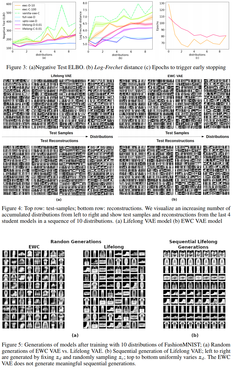
We observe that our model is comparable to the EWC baseline in this setting, however disentangles the feature space in a meaningful way (Figure 5(b)).
Sequential Permuted MNIST
Permuted MNIST is a standard dataset used in classification based continual learning works such as EWC. We extend it here to a generative setting. We observe the entire MNIST distribution at each distribution transition: the key difference being that the entire dataset undergoes a fixed permutation at each new interval.
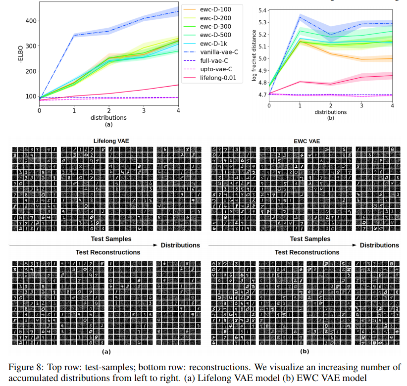
Our model drastically outperforms EWC in this scenario. We hypothesize this is due to the fact that EWC utilizes a local estimate of the KL divergence. Note that the KL divergence can be locally approximated as a quadratic difference [16]. In addition, our model regularizes the output latent variables, whereas EWC directly regularizes the parameters. Assuming a simplistic parametric form for the parameter-posterior \(P(\theta | x)\) (which EWC does) has been shown [17] to be a flawed assumption. We show that in cases where the distribution transitions to a vastly different distribution (i.e. non domain-adaptation) that our model drastically outperforms EWC (Figures 8a, 8b).
SVHN \(\mapsto\) MNIST:
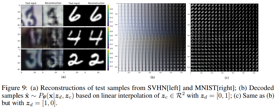 In this experiment we show that our model learns a continuous latent space suitable for both SVHN and MNIST; we consider a two-distribution scenario where we observe the entire MNIST dataset, followed by the entire SVHN dataset.
Conclusion:
We believe there is still a long road to solving the continual / lifelong learning problem. In our recent work we attempt to mitigate the effects through a novel replay mechanism coupled with a bayesian update rule. Our paper is available on arxiv for further details.
[1] Sebastian Thrun. 1998. Lifelong Learning Algorithms. In S Thrun and L Pratt, editors, Learning To Learn, pages 181–209. Kluwer Academic Publishers. [2] Szegedy, Christian, et al. "Rethinking the inception architecture for computer vision." Proceedings of the IEEE conference on computer vision and pattern recognition. 2016. [3] He, Kaiming, et al. "Deep residual learning for image recognition." Proceedings of the IEEE conference on computer vision and pattern recognition. 2016. [4] Sutskever, Ilya, Oriol Vinyals, and Quoc V. Le. "Sequence to sequence learning with neural networks." Advances in neural information processing systems. 2014. [5] Bottou, Léon (1998). "Online Algorithms and Stochastic Approximations". Online Learning and Neural Networks. Cambridge University Press. ISBN 978-0-521-65263-6 [6] T. Broderick, N. Boyd, A. Wibisono, A. C. Wilson, and M. I. Jordan. Streaming variational bayes. In C. J. C. Burges, L. Bottou, Z. Ghahramani, and K. Q. Weinberger, editors, Advances in Neural Information Processing Systems 26: 27th Annual Conference on Neural Information Processing Systems 2013. Proceedings of a meeting held December 5-8, 2013, Lake Tahoe, Nevada, United States., pages 1727–1735, 2013. [7] McCloskey, Michael and Cohen, Neal J. Catastrophic interference in connectionist networks: The sequential learning problem. Psychology of learning and motivation, 24:109–165, 1989. [8] Farquhar, Sebastian, and Yarin Gal. "Towards Robust Evaluations of Continual Learning." arXiv preprint arXiv:1805.09733 (2018). [9] C. V. Nguyen, Y. Li, T. D. Bui, and R. E. Turner. Variational continual learning. ICLR, 2018. [10] J. Kirkpatrick, R. Pascanu, N. Rabinowitz, J. Veness, G. Desjardins, A. A. Rusu, K. Milan, J. Quan, T. Ramalho, A. Grabska-Barwinska, et al. Overcoming catastrophic forgetting in neural networks. Proceedings of the National Academy of Sciences, page 201611835, 2017. [11] Z. Li and D. Hoiem. Learning without forgetting. In European Conference on Computer Vision, pages 614–629. Springer, 2016. [12] Silver, Daniel L., Qiang Yang, and Lianghao Li. "Lifelong Machine Learning Systems: Beyond Learning Algorithms." AAAI Spring Symposium: Lifelong Machine Learning. Vol. 13. 2013. [13] Rusu, Andrei A., et al. "Progressive neural networks." arXiv preprint arXiv:1606.04671 (2016). [14] F. Huszar. Infogan: using the variational bound on mutual information (twice), Aug 2016. [15] M. Heusel, H. Ramsauer, T. Unterthiner, B. Nessler, and S. Hochreiter. Gans trained by a two time-scale update rule converge to a local nash equilibrium. In Advances in Neural Information Processing Systems, pages 6629–6640, 2017. [16] Jeffreys, H. (1946). An invariant form for the prior probability in estimation problems. Proc. Royal Soc. of London, Series A, 186, 453–461. [17] Blundell, Charles, et al. "Weight uncertainty in neural networks." Proceedings of the 32nd International Conference on International Conference on Machine Learning-Volume 37. JMLR. org, 2015. [18] Chen, Xi, et al. "Infogan: Interpretable representation learning by information maximizing generative adversarial nets." Advances in neural information processing systems. 2016.